


As usual in computing, great power implies at least a bit of complexity. This 2-part article fills the gap by explaining exactly how materialized views work so that even beginners can use them effectively. We’ll work a couple of detailed examples that you can adapt to your own uses. Along the way we explore the exact meaning of syntax used to create views as well as give you insight into what ClickHouse is doing underneath. Samples are completely self-contained, so you can copy/paste them into the clickhouse-client and run them yourself.
Part-1 Basic
Computing Sums
ClickHouse materialized views automatically transform data between tables. They are like triggers that run queries over inserted rows and deposit the result in a second table. Let’s look at a basic example. Suppose we have a table to record user downloads that looks like the following.
CREATE TABLE download (
  when DateTime,
  userid UInt32,
  bytes Float32
) ENGINE=MergeTree
PARTITION BY toYYYYMM(when)
ORDER BY (userid, when)
We would like to track daily downloads for each user. Let’s see how we could do this with a query. First, we need to add some data to the table for a single user.
INSERT INTO download
  SELECT
    now() + number * 60 as when,
    25,
    rand() % 100000000
  FROM system.numbers
  LIMIT 5000
Next, let’s run a query to show daily downloads for that user. This will also work properly as new users are added.
SELECT
  toStartOfDay(when) AS day,
  userid,
  count() as downloads,
  sum(bytes) AS bytes
FROM download
GROUP BY userid, day
ORDER BY userid, day
┌─────────────────day─┬─userid─┬─downloads─┬───────bytes─┐
│ 2019-09-04 00:00:00 	│     25 │       656 │ 33269129531  │
│ 2019-09-05 00:00:00 	│     25 │      1440 │ 70947968936  │
│ 2019-09-06 00:00:00 	│     25 │      1440 │ 71590088068  │
│ 2019-09-07 00:00:00 	│     25 │      1440 │ 72100523395  │
│ 2019-09-08 00:00:00 	│     25 │        24 │  1141389078  │
└─────────────────────┴───────┴──────────┴─────────────┘
We could compute these daily totals interactively for applications by running the query each time, but for large tables it is faster and more resource efficient to compute them in advance. It would therefore be better to have the results in a separate table that continuously tracks the sum of each user’s downloads by day. We can do exactly that with the following materialized view.
CREATE MATERIALIZED VIEW download_daily_mv
ENGINE = SummingMergeTree
PARTITION BY toYYYYMM(day) ORDER BY (userid, day)
POPULATE
AS SELECT
  toStartOfDay(when) AS day,
  userid,
  count() as downloads,
  sum(bytes) AS bytes
FROM download
GROUP BY userid, day
There are three important things to notice here. First, materialized view definitions allow syntax similar to CREATE TABLE, which makes sense since this command will actually create a hidden target table to hold the view data. We use a ClickHouse engine designed to make sums and counts easy: SummingMergeTree. It is the recommended engine for materialized views that compute aggregates.
Second, the view definition includes the keyword POPULATE. This tells ClickHouse to apply the view to existing data in the download table as if it were just inserted. We’ll talk more about automatic population in a bit.
Third, the view definition includes a SELECT statement that defines how to transform data when loading the view. This query runs on new data in the table to compute the number of downloads and total bytes per userid per day. It’s essentially the same query as we ran interactively, except in this case the results will be put in the hidden target table. We can skip sorting, since the view definition already ensures the sort order.
Now let’s select directly from the materialized view.
SELECT * FROM download_daily_mv
ORDER BY day, userid
LIMIT 5
┌─────────────────day─┬─userid─┬─downloads─┬───────bytes─┐
│ 2019-09-04 00:00:00 	│     25 │       656 │ 33269129531  │
│ 2019-09-05 00:00:00 	│     25 │      1440 │ 70947968936  │
│ 2019-09-06 00:00:00 	│     25 │      1440 │ 71590088068  │
│ 2019-09-07 00:00:00 	│     25 │      1440 │ 72100523395  │
│ 2019-09-08 00:00:00 	│     25 │        24 │  1141389078  │
└─────────────────────┴───────┴──────────┴─────────────┘
This gives us exactly the same answer as our previous query. The reason is the POPULATE keyword introduced above. It ensures that existing data in the source table automatically loads into the view. There’s an important caveat however: if new data are INSERTed while the view populates, ClickHouse will miss them. We’ll show how to insert data manually and avoid missed data problems in the second part of this series.
Now try adding more data to the table with a different user.
INSERT INTO download
  SELECT
    now() + number * 60 as when,
    22,
    rand() % 100000000
  FROM system.numbers
  LIMIT 5000
If you select from the materialized view you’ll see that it now has totals for userid 22 as well as 25. Notice that the new data is available instantly–as soon as the INSERT completes the view is populated. This is an important feature of ClickHouse materialized views that makes them very useful for real-time analytics.
Here’s the query and new results.
SELECT * FROM download_daily_mv ORDER BY userid, day
┌─────────────────day─┬─userid─┬─downloads─┬───────bytes─┐
│ 2019-09-04 00:00:00 	│     22 │       654 │ 31655571524  │
│ 2019-09-05 00:00:00 	│     22 │      1440 │ 71514547751  │
│ 2019-09-06 00:00:00 	│     22 │      1440 │ 71839871989  │
│ 2019-09-07 00:00:00 	│     22 │      1440 │ 70915563752  │
│ 2019-09-08 00:00:00 	│     22 │        26 │  1227350921  │
│ 2019-09-04 00:00:00 	│     25 │       656 │ 33269129531  │
│ 2019-09-05 00:00:00 	│     25 │      1440 │ 70947968936  │
│ 2019-09-06 00:00:00 	│     25 │      1440 │ 71590088068  │
│ 2019-09-07 00:00:00 	│     25 │      1440 │ 72100523395  │
│ 2019-09-08 00:00:00 	│     25 │        24 │  1141389078  │
└─────────────────────┴───────┴──────────┴─────────────┘
As an exercise you can run the original query against the source download table to confirm it matches the totals in the view.
As a final example, let’s use the daily view to select totals by month. In this case we treat the daily view like a normal table and group by month as follows. We’ve added the WITH TOTALS clause which prints a handy summation of the aggregates.
SELECT
    toStartOfMonth(day) AS month,
    userid,
    sum(downloads),
    sum(bytes)
FROM download_daily_mv
GROUP BY userid, month WITH TOTALS
ORDER BY userid, month
┌──────month─┬─userid─┬─sum(downloads)─┬───sum(bytes)─┐
│ 2019-09-01 	│     22 │           5000 │ 247152905937  │
│ 2019-09-01 	│     25 │           5000 │ 249049099008  │
└────────────┴───────┴───────────────┴─────────────┘
Totals:
┌──────month─┬─userid─┬─sum(downloads)─┬───sum(bytes)─┐
│ 0000-00-00 	│      0 │          10000 │ 496202004945  │
└────────────┴───────┴───────────────┴─────────────┘
From the foregoing examples we can clearly see how the materialized view correctly summarizes data from the source data. We can even “summarize the summaries,” as the last example shows. So what exactly is going on under the covers? The following picture illustrates the logical flow of data.
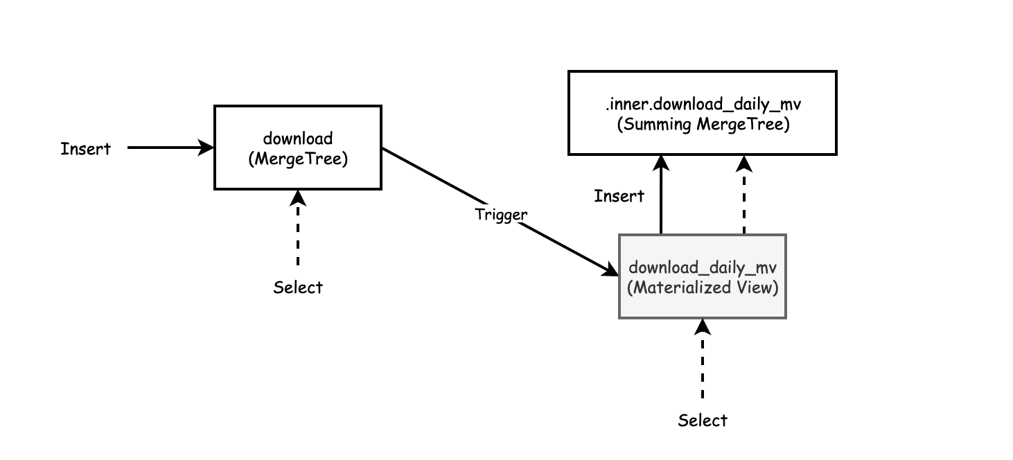
As the diagram shows, values from INSERT on the source table are transformed and applied to the target table. To populate the view all you do is insert values into the source table.
You can select from the target table as well as the materialized view. Selecting from the
materialized view passes through to the internal table that the view created automatically.
There’s one other important thing to notice from the diagram. The materialized view creates a private table with a special name to hold data. If you delete the materialized view by typing ‘DROP TABLE download_daily_mv’ the private table disappears. If you need to change the view you will need to drop it and recreate with new data.
Wrap-up
The example we just reviewed uses SummingMergeTree to create a view to add up daily user downloads. We used standard SQL syntax on the SELECT from the materialized view. This is a special capability of the SummingMergeTree engine and only works for sums and counts. For other types of aggregates we need to use a different approach.
Also, our example used the POPULATE keyword to publish existing table data into the private target table created by the view. If new INSERT rows arrive while the view is being filled ClickHouse will miss them. This limitation is easy to work around when you are the only person using a data set but problematic for production systems that constantly load data. Also, the private table goes away when the view is dropped. That makes it difficult to alter the view to accommodate schema changes in the source table.
In the next article we will show how to create materialized views that compute other kinds of aggregates like averages or max/min. We’ll also show how to define the target table explicitly and load data into it manually using our own SQL statements. We’ll touch briefly on schema migration as well. Meanwhile, we hope you have enjoyed this brief introduction and found the examples useful.
Part-2 Advance
In Part-1, we introduced a way to construct ClickHouse materialized views that compute sums and counts using the SummingMergeTree engine. The SummingMergeTree can use normal SQL syntax for both types of aggregates. We also let the materialized view definition create the underlying table for data automatically. Both of these techniques are quick but have limitations for production systems.
In the current post we will show how to create a materialized view with a range of aggregate types on an existing table. This appproach is suitable when you need to compute more than simple sums. It’s also handy for cases where your table has large amounts of arriving data or has to deal with schema changes.
Using State Functions and TO Tables to Create More Flexible Views
In the following example we are going to measure readings from devices. Let’s start with a table definition.
CREATE TABLE counter (
  when DateTime DEFAULT now(),
  device UInt32,
  value Float32
) ENGINE=MergeTree
PARTITION BY toYYYYMM(when)
ORDER BY (device, when)
Next we add sufficient data to make query times slow enough to be interesting: 1 billion rows of synthetic data for 10 devices. Note: If you are trying these out you can just put in a million rows to get started. The examples work regardless of the amount of data.
INSERT INTO counter
  SELECT
    toDateTime('2015-01-01 00:00:00') + toInt64(number/10) AS when,
    (number % 10) + 1 AS device,
    (device * 3) +  (number/10000) + (rand() % 53) * 0.1 AS value
  FROM system.numbers LIMIT 1000000
Now let’s look at a sample query we would like to run regularly. It summarizes all data for all devices over the entire duration of sampling. In this case that means 3.25 years worth of data from the table, all of it prior to 2019.
SELECT
    device,
    count(*) AS count,
    max(value) AS max,
    min(value) AS min,
    avg(value) AS avg
FROM counter
GROUP BY device
ORDER BY device ASC
. . .
10 rows in set. Elapsed: 2.709 sec. Processed 1.00 billion rows, 8.00 GB (369.09 million rows/s., 2.95 GB/s.)
The preceding query is slow because it must read all of the data in the table to get answers. We want to design a materialized view that reads a lot less data. It turns out that if we define a view that summarizes data on a daily basis, ClickHouse will correctly aggregate the daily totals across the entire interval.
Unlike our previous simple example we will define the target table ourselves. This has the advantage that the table is now visible, which makes it easier to load data as well as do schema migrations. Here’s the target table definition.
CREATE TABLE counter_daily (
  day DateTime,
  device UInt32,
  count UInt64,
  max_value_state AggregateFunction(max, Float32),
  min_value_state AggregateFunction(min, Float32),
  avg_value_state AggregateFunction(avg, Float32)
)
ENGINE = SummingMergeTree()
PARTITION BY tuple()
ORDER BY (device, day)
The table definition introduces a new datatype, called an aggregate function, which holds partially aggregated data. The type is required for aggregates other than sums or counts. Next we create the corresponding materialized view. It selects from counter (the source table) and sends data to counter_daily (the target table) using special TO syntax in the CREATE statement. Where the table has aggregate functions, the SELECT statement has matching functions like ‘maxState’. We’ll get into how these are related when we discuss aggregate functions in detail.
CREATE MATERIALIZED VIEW counter_daily_mv
TO counter_daily
AS SELECT
    toStartOfDay(when) as day,
    device,
    count(*) as count,
    maxState(value) AS max_value_state,
    minState(value) AS min_value_state,
    avgState(value) AS avg_value_state
FROM counter
WHERE when >= toDate('2019-01-01 00:00:00')
GROUP BY device, day
ORDER BY device, day
The TO keyword lets us point to our target table but has a disadvantage. ClickHouse does not allow use of the POPULATE keyword with TO. To begin with the materialized view therefore has no data. We’re going to load data manually. But we’ll also use a nice trick that enables us to avoid problems in case there is active data loading going on at the same time.
Notice that the view definition has a WHERE clause. This says that any data prior to 2019 should be ignored. We now have a way to handle data loading in a way that does not lose data. The view will take care of new data arriving in 2019. Meanwhile we can load old data from 2018 and before with an INSERT.
Let’s demonstrate how this works by loading new data into the counter table. The new data will start in 2019 and should load into the view automatically.
INSERT INTO counter
  SELECT
    toDateTime('2019-01-01 00:00:00') + toInt64(number/10) AS when,
    (number % 10) + 1 AS device,
    (device * 3) +  (number / 10000) + (rand() % 53) * 0.1 AS value
  FROM system.numbers LIMIT 10000000
Now let’s manually load the older data using the following INSERT. It loads all data from 2018 and before.
INSERT INTO counter_daily
SELECT
  toStartOfDay(when) as day,
  device,
  count(*) AS count,
  maxState(value) AS max_value_state,
  minState(value) AS min_value_state,
  avgState(value) AS avg_value_state
FROM counter
WHERE when < toDateTime('2019-01-01 00:00:00')
GROUP BY device, day
ORDER BY device, day
We are finally ready to select data out of the view. As with the target table and materialized view, ClickHouse uses specialized syntax to select from the view.
SELECT
  device,
  sum(count) AS count,
  maxMerge(max_value_state) AS max,
  minMerge(min_value_state) AS min,
  avgMerge(avg_value_state) AS avg
FROM counter_daily
GROUP BY device
ORDER BY device ASC
┌─device─┬────count─┬───────max─┬─────min─┬──────────────avg─┐
│      1 │ 101000000 │  100008.17 │   3.008 │  49515.50042561026 │
│      2 │ 101000000 │ 100011.164 │  6.0031 │ 49518.500627177054 │
│      3 │ 101000000 │  100014.17 │  9.0062 │  49521.50087863756 │
│      4 │ 101000000 │  100017.04 │ 12.0333 │   49524.5006612177 │
│      5 │ 101000000 │  100020.19 │ 15.0284 │  49527.50092650661 │
│      6 │ 101000000 │  100023.15 │ 18.0025 │  49530.50098047898 │
│      7 │ 101000000 │ 100026.195 │ 21.0326 │  49533.50099656529 │
│      8 │ 101000000 │  100029.18 │ 24.0297 │  49536.50119239665 │
│      9 │ 101000000 │ 100031.984 │ 27.0258 │  49539.50119958179 │
│     10 │ 101000000 │  100035.17 │ 30.0229 │ 49542.501308345716 │
└───────┴──────────┴───────────┴────────┴───────────────────┘
10 rows in set. Elapsed: 0.003 sec. Processed 11.70 thousand rows, 945.49 KB (3.76 million rows/s., 304.25 MB/s.)
This query properly summarizes all data including the new rows. You can check the math by rerunning the original SELECT on the counter table. The difference is that the materialized view returns data around 900 times faster. It’s worth learning a bit of new syntax to get this!!
At this point we can circle back and explain what’s going on under the covers.
Aggregate Functions
Aggregate functions are like collectors that allow ClickHouse to build aggregates from data spread across many parts. The following diagram shows how this works to compute averages. We start with a selectable value in the source table. The materialized view converts the data into a partial aggregate using the avgState function, which is an internal structure. Finally, when selecting data out, apply avgMerge to total up the partial aggregates into the resulting number.
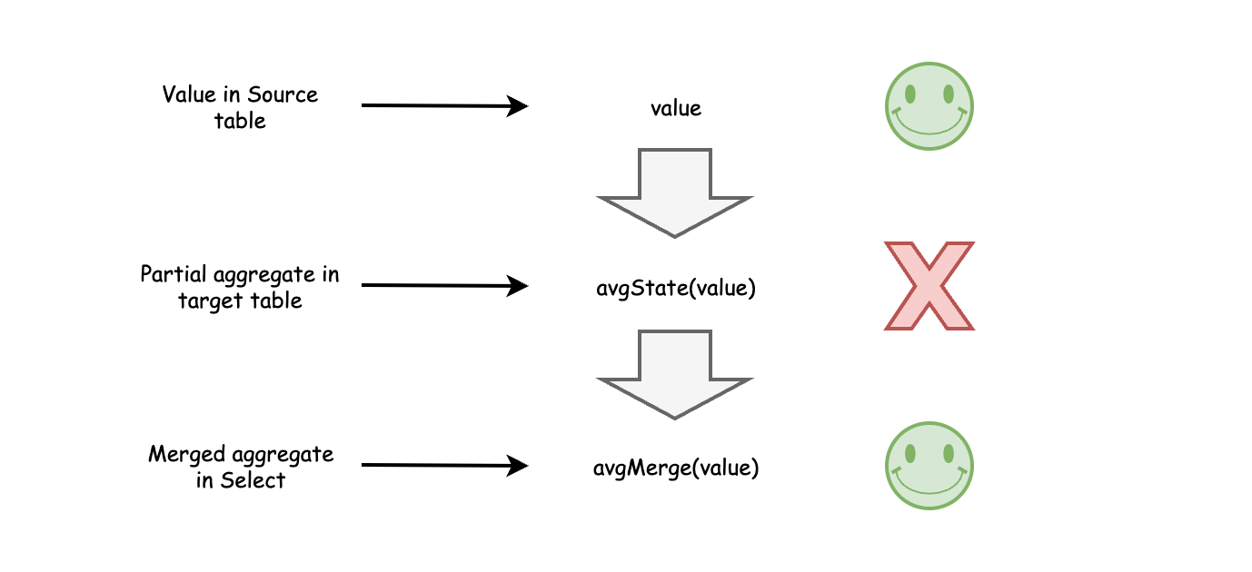
Partial aggregates enable materialized views to work with data spread across many parts on multiple nodes. The merge function properly assembles the aggregates even if you change the group by variables. It would not work just to combine simple average values, because they would be lacking the weights necessary to scale each partial average as it added to the total. This behavior has an important consequence.
Remember above when we mentioned that ClickHouse could answer our sample query using a materialized view with summarized daily data? That’s a consequence of how aggregate functions work. It means that our daily view can also answer questions about the week, month, year, or entire interval.
ClickHouse is somewhat unusual that it directly exposes partial aggregates in the SQL syntax, but the way they work to solve problems is extremely powerful. When you design materialized views try to use tricks like daily summarization to solve multiple problems with a single view. A single view can answer a lot of questions.
Table Engines for Materialized Views
ClickHouse has multiple engines that are useful for materialized views. The AggregatingMergeTree engine works with aggregate functions only. If you want to do counts or sums you’ll need to define them using AggregateFunction datatypes in the target table. You’ll also need to use state and merge functions in the view and select statements. For example, to process counts you would need to use countState(count) and countMerge(count) in our worked examples above.
We recommend the SummingMergeTree engine to do aggregates in materialized views. It can handle aggregate functions perfectly well. However it hides them for sums and counts, which is handy for simple cases. It does not prevent you from using the state and merge functions in this case; it’s just you don’t have to. Meanwhile it does everything that AggregatingMergeTree does.
Schema Migration
Database schema tends to change in production systems, especially those that are under active development. You can manage such changes relatively easily when using materialized views with an explicit target table.
Let’s take a simple example. Suppose the name of the counter table changes to counter_replicated. The materialized view won’t work once this change is applied. Even worse, the failures will block INSERTs to the counter table. You can deal with the change as follows.
-- Delete view prior to schema change.
DROP TABLE counter_daily_mv
-- Rename source table.
RENAME TABLE counter TO counter_replicated
-- Recreate view with correct source table name.
CREATE MATERIALIZED VIEW counter_daily_mv
TO counter_daily
AS SELECT
  toStartOfDay(when) as day,
  device,
  count(*) as count,
  maxState(value) AS max_value_state,
  minState(value) AS min_value_state,
  avgState(value) AS avg_value_state
FROM counter_replicated
GROUP BY device, day
ORDER BY device, day
Depending on the actual steps in schema migration you may have to work around missed data that arrives while the materialized view definition is being changed. You can handle that using filter conditions and manual loading as we showed in the main example.
Materialized View Plumbing and Data Sizes
Finally, let’s look again at the relationship between the data tables and the materialized view. The target table is a normal table. You can select data from either the target table or the materialized view. There is no difference. Moreover, if you drop the materialized view, the table remains. As we just showed, you can make schema changes to the view by simply dropping and recreating it. If you need to change the target table itself, run ALTER TABLE commands as you would for any other table.
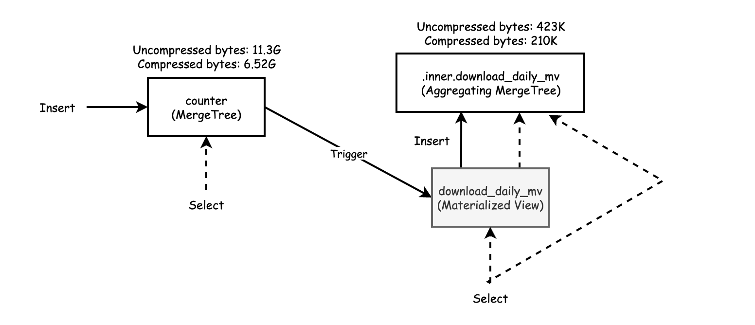
The diagram also shows the data size of the source and target tables. Materialized views are often vastly smaller than the tables whose data they aggregate. That’s certainly the case here. The following query shows the difference in sizes for this example.
SELECT
  table,
  formatReadableSize(sum(data_compressed_bytes)) AS tc,
  formatReadableSize(sum(data_uncompressed_bytes)) AS tu,
  sum(data_compressed_bytes) / sum(data_uncompressed_bytes) AS ratio
FROM system.columns
WHERE database = currentDatabase()
GROUP BY table
ORDER BY table ASC
┌─table────────────┬─tc─────────┬─tu─────────┬──────────────ratio─┐
│ counter          	│ 6.52 GiB   	│ 11.29 GiB  	│ 0.5778520850660066 	 │
│ counter_daily    	│ 210.35 KiB 	│ 422.75 KiB 	│ 0.4975675675675676 	 │
│ counter_daily_mv 	│ 0.00 B     	│ 0.00 B     	│                nan 	 │
└─────────────────┴────────────┴────────────┴────────────────────┘
As the calculations show, the materialized view target table is approximately 30,000 times smaller than the source data from which the materialized view derives. This difference speeds up queries enormously. As we showed earlier our test query runs about 900x faster when using data from the materialized view.
Wrap-up
ClickHouse materialized views are extremely flexible, thanks to powerful aggregate functions as well as the simple relationship between source table, materialized view, and target table. The fact that materialized views allow an explicit target table is a useful feature that makes schema migration simpler. You can also mitigate potential lost view updates by adding filter conditions to the view SELECT definition and manually loading missed data.
Finally, if you are using materialized views in a way you think would be interesting to other users, write an article or present at a local ClickHouse meetup.
评论区